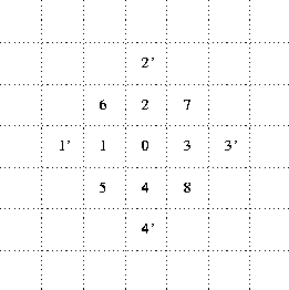
Figure 1: Numbering of Neighbor Positions
 4.2 Algorithm
 4 Internal Algorithm Review
 4 Internal Algorithm Review
This section of (Varela et al. 1974) first defines alphanumeric codes for the distinct chemical species or ``elements'' in the model. These are the same codes already introduced above, with the addition of a separate code for bonded links (BL); However, notwithstanding this, the term ``link'', denoted L, is still usually explicitly qualified as either ``free'', ``singly bonded'' or ``doubly bonded''. In fact, the code BL is used only twice by Varela et al. in the subsequent discussion and definition of the algorithm. Since bonded links are otherwise generally regarded as simply link particles with bonds (rather than another distinct kind of element) I will generally dispense with the BL code.
Next, the overall structure of the algorithm is described as consisting of two separate phases, the first concerned with movement, the second with the various reactions. A final comment here is that ``...[t]he rules by which L components bond to form a boundary complete the algorithm''; this is a somewhat unfortunate phrasing because it prejudges the issue of whether bonding will actually lead to closed chains (``boundaries'').
The discrete space, with a rectangular co-ordinate system, or square lattice, is described next. It is specified that the initial state of the space should contain one or more K particles, but otherwise be completely filled by S. It is unclear to me why this restriction is imposed; in any case, one would expect any comprehensive computer implementation to allow arbitrary initialisation of the particles in the space (and, indeed, subsequent intervention and manipulation of it).
Both movement and reactions depend, in part, on the relative spatial positions of the interacting particles; so a convention for labeling relative (``neighborhood'') positions in the space is introduced next. Figure 1 is a redrawn version of this scheme (drawn in terms of lattice cells rather than lattice points as in the original paper). Notice, in particular, that the neighborhood extends two positions away from the central cell, but only in the orthogonal (not diagonal) directions. This is an essential device to support S particles permeating through chains of L.

Figure 1: Numbering of Neighbor Positions
The only comment about behaviour at the edges of the space occurs parenthetically in the discussion of this neighborhood diagram:
...of course, near the array boundaries, not all of the neighbor locations identified in the figure will actually be found...
I interpret this to mean, as earlier indicated, that the edges are to be regarded as hard limits to the space--no interactions or motions can operate beyond these edges. This is in contrast to, say, making the space effectively toroidal, so that cells on the East edge are considered adjacent to the West edge, and similarly for the North and South edges. I suggest that the latter arrangement might actually be conceptually preferable, because the edges otherwise introduce an asymmetry into the space, which may give rise to artifact phenomena.
There follows a qualitative discussion of motion in the model. This is expressed in terms of the particles being ``ranked'' by ``mass'', where ``mass'' here denotes which kinds of particles may displace which others. This is, at best, a relatively weak analog of newtonian mass, and there are no analogs of force, momentum, energy etc. All motion in the space is fundamentally a form of simple diffusion or random walk.
Roughly speaking then, the ranking by increasing mass is in the order S, (free) L, K; so K particles can displace, or push away, free L and S particles, free L particles can displace S particles, and S particles can only move into holes. Bonded L particles cannot move at all. S may move through a single thickness chain of bonded L particles, but free L and K particles cannot.
The algorithm proper fleshes out these motion rules more precisely. However, I should note here that this idea of ranking by ``mass'', with the possibility of ``displacement'', does complicate the algorithm very substantially and yet seems to me to contribute little if anything to the utility of the model. The rules on permeability of chains of L particles are clearly crucial to the possibility of autopoietic organisation being realised-but that is a completely separate issue from whether certain particles are ranked by ``mass'' or can ``displace'' other particles. If the idea was to implement varying degrees of mobility for the different kinds of particles, I suggest this could have been more simply achieved by qualifying the motions by a probability (of ``attempted'' motion), per particle, per timestep. In any case, I conjecture that the relatively complicated model of motion actually proposed by Varela et al. does not significantly affect the capacity for the model to support autopoietic phenomena.
Next comes a qualitative discussion of the production reaction, specifying that the two S particles must be immediately adjacent to each other and to a K particle. Thus, taking the K to be in the centre of a neighborhood (position 0 of figure 1), the S particles might be in relative positions 2 and 7, or 5 and 4, but not 1 and 3, etc. It is explicitly stipulated here that the reaction rate is limited to, at most, production of one L per K per timestep. If there are multiple pairs of S particles which could react under the action of a given K in one timestep, then one pair is to be selected at ``random''. Since the production reaction consumes two S particles to produce one L particle, it also results, in effect, in production of an additional hole in the space--into which particles may subsequently diffuse.
The final paragraph of this section is concerned with the disintegration reaction and will be quoted in full:
The disintegration of L's is applied as a uniform probability of disintegration per timestep for each L whether bonded or free, which results in a proportionality between failure rate and size of a chain structure. The sharply limited rate of ``repair'', which depends upon random motion of S's through the membrane, random production of new L's and random motion to the repair site, makes the disintegration a very powerful controller of the maximum size for a viable boundary structure. A disintegration probability of less than about .01 per timestep is required in order to achieve any viable structure at all (these must contain roughly ten L units at least to form a closed structure with any space inside).
This introduces the only explicitly specified parameter
of the model (subsequently labeled ![]() ), being the
probability of disintegration per L particle
(bonded or otherwise) per timestep. The implication
is that this is the only behaviour or interaction in
the model which will be characterised by such a rate
parameter; one must presume, therefore, that the other
dynamics are intended to proceed at the ``maximum''
rate (consistent with any explicitly stated constraints
or enabling conditions). Thus, all particles
will move whenever they can; S
particles will react (under the action of K)
whenever they can; L particles will form
additional bonds whenever they can.
), being the
probability of disintegration per L particle
(bonded or otherwise) per timestep. The implication
is that this is the only behaviour or interaction in
the model which will be characterised by such a rate
parameter; one must presume, therefore, that the other
dynamics are intended to proceed at the ``maximum''
rate (consistent with any explicitly stated constraints
or enabling conditions). Thus, all particles
will move whenever they can; S
particles will react (under the action of K)
whenever they can; L particles will form
additional bonds whenever they can.
It is clear that the model could be easily generalised by introducing new rate parameters (effectively, probabilities of the action, per site, per unit time), analogous to the disintegration rate parameter. Setting these parameters to 1 would then recover precisely the model explicitly specified by Varela et al. (1974). The ``mobility'' probabilities mentioned earlier are specific examples of this. I suggest, therefore, that a computer implementation of the model should support such additional parameters, thus allowing a wider range of models, and corresponding phenomenology, to be explored. These potential additional parameters will be elaborated below in the detailed discussion of the algorithm proper.
The final point to be made here is that while Varela
et al. stipulate that ![]() should be less than 0.01
(which would yield a composite probability of
disintegration for a 10 particle L chain of just
under 0.1, or an expected lifetime, for the chain, of
about 10 timesteps), they do not say precisely how
much less. Clearly, the phenomenology of the
model will alter as this parameter is made smaller;
thus, it would have been useful to specify what precise
value(s) were used in the particular experiments
reported in the paper.
should be less than 0.01
(which would yield a composite probability of
disintegration for a 10 particle L chain of just
under 0.1, or an expected lifetime, for the chain, of
about 10 timesteps), they do not say precisely how
much less. Clearly, the phenomenology of the
model will alter as this parameter is made smaller;
thus, it would have been useful to specify what precise
value(s) were used in the particular experiments
reported in the paper.
 4.2 Algorithm
 4 Internal Algorithm Review
 4 Internal Algorithm Review
Copyright © 1997 All Rights Reserved.
Timestamp: Tue Dec 31 18:43:32 GMT 1996